Developing and maintaining a DNA reference database can be difficult.
The refdb package has been developed to assist you during
the different steps of the process of developing, maintaining and using
DNA reference databases efficiently and reproducibly. This vignette will
present some of the important functions of the package and help you to
get started with it.
Installing and loading the package
The refdb package is available on CRAN, which means that you can
easily install the latest stable version using the RStudio IDE or with
the function install.packages. In this tutorial we will
also be using functions from several packages of the tidyverse.
Therefore, if the tidyverse package is not already
installed on your computer, you are encouraged to install it now.
Once everything is ready, we can start by loading the packages we need:
Reading data
Reading data from a file
In refdb, a reference database is a simple dataframe.
This means that any functions able to read external data and return a
dataframe in your R environment can be used to import a reference
library. Here, for simplicity, we will assume the reference database is
stored as a CSV on your computer’s local harddrive. You can download the
example file here
(use “Save as”). Then, we can read the file from its location on your
computer with:
lib <- read_csv("my_path/ephem.csv")Note that we use the function read_csv from tidyverse,
which returns a tibble. A tibble is a dataframe with some extra
refinements. There is no issue with using tibbles with refdb functions
(this is actually encouraged).
Setting fields
Now we have a dataframe (a tibble) in our environment. However, the
functions of the refdb package can’t use it directly, as first the
actual content stored in each column has to be specified. You have to
provide this information, and this can be done using the function
refdb_set_fields:
lib <- refdb_set_fields(lib,
                        taxonomy = c(family = "family_name",
                                     genus = "genus_name",
                                     species = "species_name"),
                        sequence = "DNA_seq",
                        marker = "marker")
Here we explicitly set the taxonomy, sequence, and marker fields by indicating which columns of the dataframe correspond to each of those fields.
If you now print the object lib, you will see that the
nucleotide symbols in the columns DNA_seq are colored. This is because
this column has been identified as containing DNA sequences. A simple
way to see which fields have been associated with which column is simply
to use the function refdb_get_fields.
refdb_get_fields(lib)
#> taxonomy:
#>   family: family_name
#>   genus: genus_name
#>   species: species_name
#> sequence: DNA_seq
#> marker: marker
Note that if you are importing data from some popular reference
databases, these functions can save you time:
refdb_set_fields_BOLD, refdb_set_fields_NCBI,
refdb_set_fields_PR2,
refdb_set_fields_diatbarcode.
Cleaning taxonomic names and DNA sequences
Once the data are loaded and the fields have been set, we can start to work with the reference database. The first thing we will look at, is how to clean taxonomic names and DNA sequences. Cleaning is different than filtering (that we will see in the next section) in that the objective here is not to remove entries, but to correct them.
Both sequences and taxonomic names can be affected by countless problems, which we do not list here all. However, the refdb package provides functions to deal with many of the common cases. Let’s review some of them.
Missing taxonomic information
Let’s take a look at the taxonomy of the 91st record:
lib [91, 1:4]
#> # A tibble: 1 × 4
#>   order_name    family_name     genus_name species_name
#>   <chr>         <chr>           <chr>      <chr>
#> 1 Ephemeroptera Leptophlebiidae Thraulodes Thraulodes sp.
Here, the specimen has been identified at the genus level and the
species is reported using the notation “sp.”. This is a common notation
but not really a practical one when you manage a database. How would you
report the family of an organism identified at the class level? In R, a
general and efficient way to code for a missing information is simply to
use the built-in NA indicator.
The function refdb_clean_tax_NA can be used to identify
taxonomic levels for which there are no information and change them to
NA:
lib_na <- refdb_clean_tax_NA(lib)
lib_na [91, 1:4]
#> # A tibble: 1 × 4
#>   order_name    family_name     genus_name species_name
#>   <chr>         <chr>           <chr>      <chr>
#> 1 Ephemeroptera Leptophlebiidae Thraulodes NA
Extra information appended to taxonomic names
It is common to find taxonomic names to which various information have been added. See the 32nd row of our database:
lib [32, 1:4]
#> # A tibble: 1 × 4
#>   order_name    family_name   genus_name species_name
#>   <chr>         <chr>         <chr>      <chr>
#> 1 Ephemeroptera Heptageniidae Epeorus    Epeorus longimanus B BG
The species name is tagged “B BG”. This extra information probably
meant something to the person who recorded this entry (e.g., some field
or identification notes), but is not useful to us and may even be
problematic. The function refdb_clean_tax_remove_extra uses
some simple rules to detect these information and remove them:
lib_na_extra <- refdb_clean_tax_remove_extra(lib_na)
lib_na_extra [32, 1:4]
#> # A tibble: 1 × 4
#>   order_name    family_name   genus_name species_name
#>   <chr>         <chr>         <chr>      <chr>
#> 1 Ephemeroptera Heptageniidae Epeorus    Epeorus longimanus
A note on false positive and false negative
The cleaning functions of refdb uses several rules and heuristics, some of them can produce false positive and false negative. You should always be careful of the functions actions. If you find cases where a function does not what it is expected to do, please report here.
Cleaning DNA sequences
Similarly, it is possible to clean the sequences with different functions. For example, if we want to remove the gaps in the sequences:
head(lib)
#> # A tibble: 6 × 8
#>   order_name    family_name  genus_name species_name marker DNA_seq   lat    lon
#>   <chr>         <chr>        <chr>      <chr>        <chr>  <DNA>   <dbl>  <dbl>
#> 1 Ephemeroptera Heptageniid… Epeorus    Epeorus fra… COI-5P ATAGTC…  39.5  -79.2
#> 2 Ephemeroptera Oligoneurii… Oligoneur… Oligoneurie… COI-5P GACTTT…  42.4   22.5
#> 3 Ephemeroptera Ephemerelli… Serratella Serratella … COI-5P ------…  34.2 -118.
#> 4 Ephemeroptera Baetidae     Fallceon   NA           COI-5P ------…  34.2 -119.
#> 5 Ephemeroptera Heptageniid… Heptagenia Heptagenia … COI-5P AACTTT…  58.7  -94.2
#> 6 Ephemeroptera Heptageniid… Epeorus    Epeorus vit… COI-5P AACTCT…  46.8  -66.1

lib_nogap <- refdb_clean_seq_remove_gaps(lib)
head(lib_nogap)
#> # A tibble: 6 × 8
#>   order_name    family_name  genus_name species_name marker DNA_seq   lat    lon
#>   <chr>         <chr>        <chr>      <chr>        <chr>  <DNA>   <dbl>  <dbl>
#> 1 Ephemeroptera Heptageniid… Epeorus    Epeorus fra… COI-5P ATAGTC…  39.5  -79.2
#> 2 Ephemeroptera Oligoneurii… Oligoneur… Oligoneurie… COI-5P GACTTT…  42.4   22.5
#> 3 Ephemeroptera Ephemerelli… Serratella Serratella … COI-5P TGAGTT…  34.2 -118.
#> 4 Ephemeroptera Baetidae     Fallceon   NA           COI-5P TAAGAT…  34.2 -119.
#> 5 Ephemeroptera Heptageniid… Heptagenia Heptagenia … COI-5P AACTTT…  58.7  -94.2
#> 6 Ephemeroptera Heptageniid… Epeorus    Epeorus vit… COI-5P AACTCT…  46.8  -66.1
Other cleaning functions
We have only seen a brief overview of the functions available for cleaning up the sequences and their associated taxonomy. Many further functions and options are possible, listed in the table below that summarizes all functions currently available in refdb:
| Function | Description |
|---|---|
| refdb_clean_seq_remove_gaps | Remove gaps from genetic sequences |
| refdb_clean_seq_remove_sideN | Remove repeated side N from genetic sequences |
| refdb_clean_seq_crop_primers | Crop genetic sequences with a set of primers |
| refdb_clean_tax_remove_blank | Remove blank characters from taxonomic names |
| refdb_clean_tax_remove_extra | Remove extra words from taxonomic names |
| refdb_clean_tax_harmonize_nomenclature | Harmonize taxonomic name nomenclature |
| refdb_clean_tax_remove_uncertainty | Remove terms indicating uncertainty in taxonomic names |
| refdb_clean_tax_remove_subsp | Remove subspecific information from taxonomic names |
| refdb_clean_tax_NA | Convert missing taxonomic names to NA |
Filtering records
Filtering is the step that usually follows cleaning and whose objective is to identify and remove records (rows) that do not satisfy quality criteria (those criteria and associated thresholds are of course specific to each project).
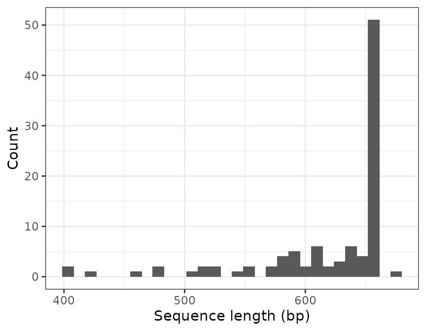
For example, we may want to exclude very short sequences whose length is likely shorter than the targeted genetic marker. Let’s take a look at the distribution of sequence lengths in the database:
refdb_plot_seqlen_hist(lib)
#> `stat_bin()` using `bins = 30`. Pick better value with `binwidth`.
To exclude all the sequences shorter than 500 nucleotides we use the
function refdb_filter_seq_length:
lib_long <- refdb_filter_seq_length(lib, min_len = 500)

nrow(lib)
#> [1] 100
nrow(lib_long)
#> [1] 94
The function has removed 6 records.
Another, more sophisticated filtering function is
refdb_filter_seq_primer(), which can find sequences that do
not contain a motif (typically a primer sequence) and remove them from
the reference database.
For example, a commonly used forward primer for metazoan is the mlCOIintF (Leray 2013). If we want to keep only the sequences where this primer is found we can use:
refdb_filter_seq_primer(lib, primer_forward = "GGWACWGGWTGAACWGTWTAYCCYCC")
#> # A tibble: 76 × 8
#>    order_name    family_name genus_name species_name marker DNA_seq   lat    lon
#>    <chr>         <chr>       <chr>      <chr>        <chr>  <DNA>   <dbl>  <dbl>
#>  1 Ephemeroptera Oligoneuri… Oligoneur… Oligoneurie… COI-5P GACTTT…  42.4   22.5
#>  2 Ephemeroptera Ephemerell… Serratella Serratella … COI-5P ------…  34.2 -118.
#>  3 Ephemeroptera Baetidae    Fallceon   NA           COI-5P ------…  34.2 -119.
#>  4 Ephemeroptera Heptagenii… Heptagenia Heptagenia … COI-5P AACTTT…  58.7  -94.2
#>  5 Ephemeroptera Heptagenii… Epeorus    Epeorus vit… COI-5P AACTCT…  46.8  -66.1
#>  6 Ephemeroptera Ephemerell… Ephemerel… Ephemerella… COI-5P AACTTT…  46.0  -66.7
#>  7 Ephemeroptera Baetidae    Baetis     Baetis huds… COI-5P CGTTAT…  67.8 -115.
#>  8 Ephemeroptera Polymitarc… Ephoron    Ephoron shi… COI-5P GAACTT…  34.1  134.
#>  9 Ephemeroptera Ephemerell… Serratella Serratella … COI-5P AACTTT…  34.2 -118.
#> 10 Ephemeroptera Ephemerell… Ephemerel… Ephemerella… COI-5P ACTTTA…  39.9  -75.8
#> # ℹ 66 more rows
You can see that only 76 sequences have passed the filter. By default
the tolerance of error is 10%. We can change this value using the
max_error_forward argument:
refdb_filter_seq_primer(lib, primer_forward = "GGWACWGGWTGAACWGTWTAYCCYCC", max_error_forward = 0.2)
#> # A tibble: 99 × 8
#>    order_name   family_name genus_name species_name marker DNA_seq   lat     lon
#>    <chr>        <chr>       <chr>      <chr>        <chr>  <DNA>   <dbl>   <dbl>
#>  1 Ephemeropte… Heptagenii… Epeorus    Epeorus fra… COI-5P ATAGTC…  39.5  -79.2
#>  2 Ephemeropte… Oligoneuri… Oligoneur… Oligoneurie… COI-5P GACTTT…  42.4   22.5
#>  3 Ephemeropte… Ephemerell… Serratella Serratella … COI-5P ------…  34.2 -118.
#>  4 Ephemeropte… Baetidae    Fallceon   NA           COI-5P ------…  34.2 -119.
#>  5 Ephemeropte… Heptagenii… Heptagenia Heptagenia … COI-5P AACTTT…  58.7  -94.2
#>  6 Ephemeropte… Heptagenii… Epeorus    Epeorus vit… COI-5P AACTCT…  46.8  -66.1
#>  7 Ephemeropte… Ephemerell… Ephemerel… Ephemerella… COI-5P AACTTT…  46.0  -66.7
#>  8 Ephemeropte… Baetidae    Baetis     Baetis huds… COI-5P CGTTAT…  67.8 -115.
#>  9 Ephemeropte… Polymitarc… Ephoron    Ephoron shi… COI-5P GAACTT…  34.1  134.
#> 10 Ephemeropte… Baetidae    Baetis     Baetis rhod… COI-5P AGCTCG…  52.2   -3.80
#> # ℹ 89 more rows
By increasing the maximum error rate to 20%, we now retain 99 sequences.
Similarly to the the cleaning functions, there are many filtering functions available in refdb, as shown in the table below:
| Function | Description |
|---|---|
| refdb_filter_seq_length | Filter sequences based on their number of characters |
| refdb_filter_seq_ambiguous | Filter sequences based on their number of ambiguous characters |
| refdb_filter_seq_homopolymers | Filter sequences based on their number of repeated characters |
| refdb_filter_seq_duplicates | Filter duplicated sequences |
| refdb_filter_seq_stopcodon | Filter sequences based on their number of stop codons |
| refdb_filter_seq_primer | Filter sequences based on the presence of primers |
| refdb_filter_tax_precision | Filter records based on their taxonomic precision |
| refdb_filter_ref_scope | Filter records by taxonomic scope of studies |
Visualizing the reference library
Now let’s take a tour of the functions you can use to produce
graphical representation of your reference database. Because refdb
stores reference database as dataframes it is straightforward to produce
plots (e.g. with the tidyverse and ggplot2). For example,
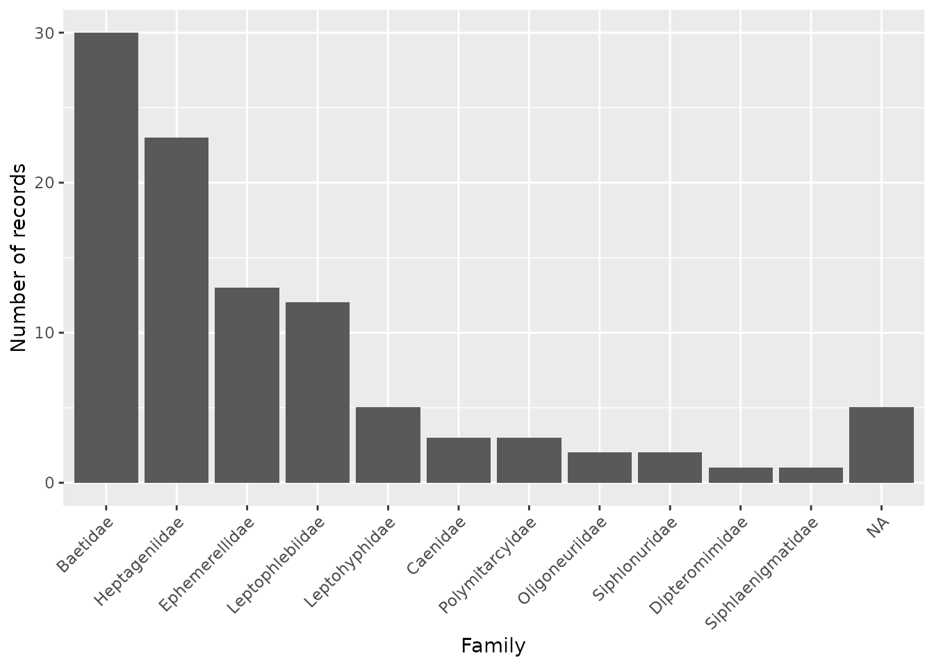
we can make a barplot showing the distribution of the families like
this:
lib %>%
  group_by(family_name) %>%
  count() %>%
  ggplot(aes(fct_reorder(family_name, n, .desc = TRUE), n)) +
  geom_col() +
  xlab("Family") +
  ylab("Number of records") +
  theme(axis.text.x = element_text(angle = 45, vjust = 1, hjust=1))
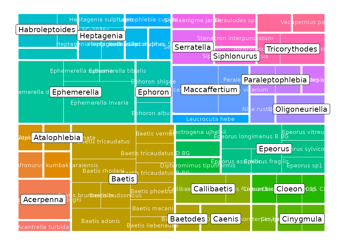
Additionally, refdb provides ready-to-use functions to produce more sophisticated plots. For example, to represent the taxonomic coverage of your reference library across multiple levels with a tree map:

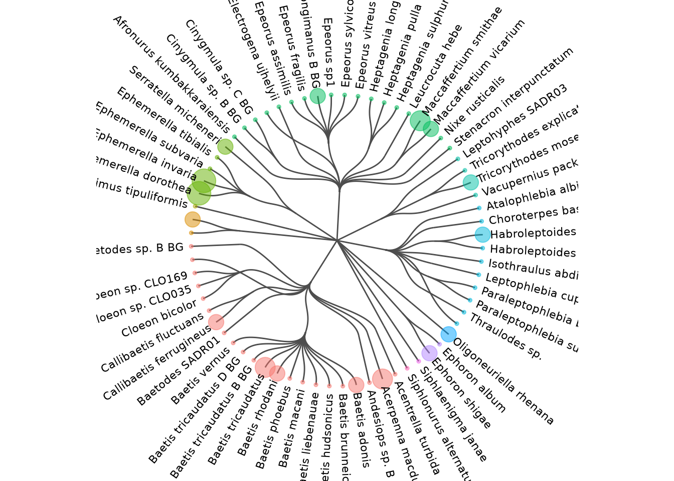
Alternatively you can represent this information with a taxonomic tree. These functions have several parameters to control what is represented in the plot (taxonomic ranks, colors, etc.).
refdb_plot_tax_tree(lib)
We conclude our overview of the graphical features of refdb with the
refdb_plot_map function, which can be used to generate
interactive maps from the data. Of course this requires the sequences to
be geographically located. As we have not yet associated columns to the
latitude and longitude fields, we have to do this beforehand:
lib <- refdb_set_fields(lib, latitude = "lat", longitude = "lon")
refdb_plot_map(lib)
Creating a report
A report is a simple and rapid way to get an overview of the current
state of your reference library and to identify some possible issues.
You can compile a report using the function
refdb_report:
refdb_report(lib)The result (not shown here) is an interactive HTML report that can be
opened in any recent web browser. It contains some statistics and plots,
and the results of functions refdb_check_tax_typo,
refdb_check_tax_conflict and
refdb_check_seq_conflict. These functions can be used to
identify possible spelling errors in taxonomic names, conflicts in the
taxonomic tree and lack of genetic resolution in sequences,
respectively.
Exporting the data
Once satisfied with the results, they can be exported for further
use. Since the reference database is a dataframe, it is possible to use
any export functions (from R or from other packages) that support
dataframes. Here we show how to export to CSV using the function
write_csv from the readr package:
write_csv(lib, "my_reference_library.csv")This will write the actual content of lib but ignore the
fields which have been previously set. We can save them in a separate
YAML file using:
refdb_write_fields(lib, "my_reference_fields.yml")Then, the next time you will open this reference database, it will be
easy to set the fields again using the argument config_yaml
of the function refdb_set_fields:
lib <- read_csv("my_reference_library.csv")
lib <- refdb_set_fields(lib, config_yaml = "my_reference_fields.yml")